XRF محلل الخوارزمية مقابل خوارزمية المعامل التجريبي

يعتقد معظم الخبراء أن خوارزمية FP تعمل عادة بشكل أفضل لاستخدامات محلل XRF. هذا صحيح عندما تحتاج إلى دقة جيدة وتثق في النتائج. تشير الدراسات إلى أن معاملات التحديد للعناصر المهمة مثل Fe, آل, و SI أعلاه 0.85. الانحرافات المعيارية النسبية أقل من 10%. هذا يعني أن النتائج دقيقة للغاية. أشياء مثل المدة التي تقيسها, الطقس, ويمكن لسطح العينة تغيير النتائج. لذا, يمكن أن يؤدي استخدام أوقات العد الأطول والتحقق من المزيد من المواقع إلى جعل النتائج أكثر موثوقية.

الوجبات الرئيسية

• ال خوارزمية FP دقيق جدا ومرن. إنه يعمل بشكل جيد مع عينات غير معروفة أو طبقات. كما أنه يعمل مع عينات معقدة. يحتاج إلى عدد أقل من معايير المعايرة.

• ال طريقة المعامل التجريبي جيد للاختبارات العادية. إنه يعمل بشكل أفضل مع العينات التي تعرفها جيدًا. يحتاج إلى العديد من المعايير المطابقة. كما يحتاج إلى معايرة دقيقة.

• استخدام كلتا الطريقتين معًا يجعل النتائج أفضل. هذا صحيح بالنسبة للعينات المعقدة. إنه يعطي دقة وثقة على مستوى المختبر.

• يجب عليك إعداد العينات ومعايرةها جيدًا. هذا مهم لكلا الخوارزميات. It helps give good XRF analysis results.

• اختر خوارزمية FP للعمل الميداني السريع والمرن. استخدم الطريقة التجريبية للاختبارات المعملية الدقيقة مع عينات ثابتة.

أيهما أفضل?

إجابة سريعة

يعتمد الاختيار بين خوارزمية FP وطريقة المعامل التجريبي على ما تحتاجه. يقول معظم الخبراء إن خوارزمية FP تعطي دقة أفضل وأكثر موثوقية بالنسبة للكثيرين محلل XRF وظائف. تستخدم خوارزمية FP النماذج المادية لإصلاح تأثيرات المصفوفة. يمكن أن تعمل مع العديد من أنواع العينات. تعتبر طريقة المعامل التجريبي مفيدًا للاختبارات الروتينية عندما تبقى مصفوفة العينة كما هي.

دراسة أجراها Ytsma et al. (2025) نظرت إلى نهج FP والتحليل التجريبي متعدد المتغيرات مع العديد من المعايير الجيولوجية. وجدت الدراسة أن النماذج التجريبية, خاصة أولئك الذين يعانون من الانحدار المتقدم, يمكن أن تتنبأ وكذلك معايرة FP. هذه النماذج أفضل أيضًا في إيجاد كميات منخفضة من العناصر. لكن الدراسة استخدمت التعلم الآلي, ليست طريقة المعامل التجريبي المعتاد. لذا, على الرغم من أن الطرق التجريبية يمكن أن تعمل بشكل جيد, the FP algorithm is still the main choice for most XRF uses.

نصيحة: إذا كنت تريد المرونة والدقة مع عينات مختلفة, عادة ما تكون خوارزمية FP هي أفضل اختيار.

العوامل الرئيسية

Some important things affect which algorithm works best for تحليل XRF. يجب على المستخدمين التفكير في هذه قبل اختيار واحدة:

• الحصول على الكمية المناسبة من العناصر مثل الحديد, نحاس, الزنك, والبوتاسيوم مطلوب للحصول على نتائج جيدة.

• يساعد تحليل XRF في العثور على كميات صغيرة من العناصر في أشياء مثل الخلايا الشمسية أو الأنسجة الحية.

• يتيح قياس العناصر الطريقة الصحيحة للعلماء توصيل البيانات بخصائص المواد.

يوضح الجدول أدناه مقاييس الأداء الرئيسية وكيف تؤثر على نتائج خوارزمية XRF:

يجب على المستخدمين أيضًا وضع هذه الأشياء في الاعتبار:

• المعايرة مهمة للغاية لكلا الخوارزميات.

• تساعد معالجات الإشارات الرقمية المتقدمة في جعل الدقة أفضل وضوضاء خلفية أقل.

• التعامل مع الأحداث المرفوضة والتراكم بالطريقة الصحيحة تجعل البيانات أكثر جدارة بالثقة.

عند الانتقاء بين خوارزمية FP وطريقة المعامل التجريبي, يجب على المستخدمين مطابقة الخوارزمية مع عينةهم, ما مدى دقةهم, وماذا معايرة الأدوات لديهم. إن اختيار الصحيح يعطي نتائج أفضل ويجعلك تثق في بيانات محلل XRF الخاص بك أكثر.

FP أساسيات خوارزمية

كيف تعمل

تستخدم خوارزمية FP الفيزياء والرياضيات لمعرفة مقدار كل عنصر في عينة. أولاً, يقيس الأشعة السينية التي تظهر عندما تضرب الشعاع العينة. ثم, يستخدم الثوابت الفيزيائية المعروفة لمعرفة مقدار كل عنصر. تُظهر هذه الثوابت كيف تتفاعل الأشعة السينية مع عناصر مختلفة. تعمل خوارزمية FP على إصلاح تأثيرات المصفوفة, التي هي التغييرات الناجمة عن عناصر أخرى في العينة. بسبب هذا, يمكن أن تعمل مع العديد من أنواع العينات, حتى لو كان مكياجهم مختلفًا.

لا تحتاج خوارزمية FP إلى العديد من المعايير للمعايرة. يستخدم القوانين الفيزيائية وعينات مرجعية قليلة. هذا يجعلها مرنة للمواد المختلفة. يستخدم العلماء خوارزمية FP في أ محلل XRF الحديث للحصول على نتائج سريعة ودقيقة.

ال يوضح الجدول أدناه كيف تتحسن خوارزمية FP في الاختبارات الحقيقية. تظهر الأرقام دقة أعلى وخطية أفضل للعناصر المهمة:

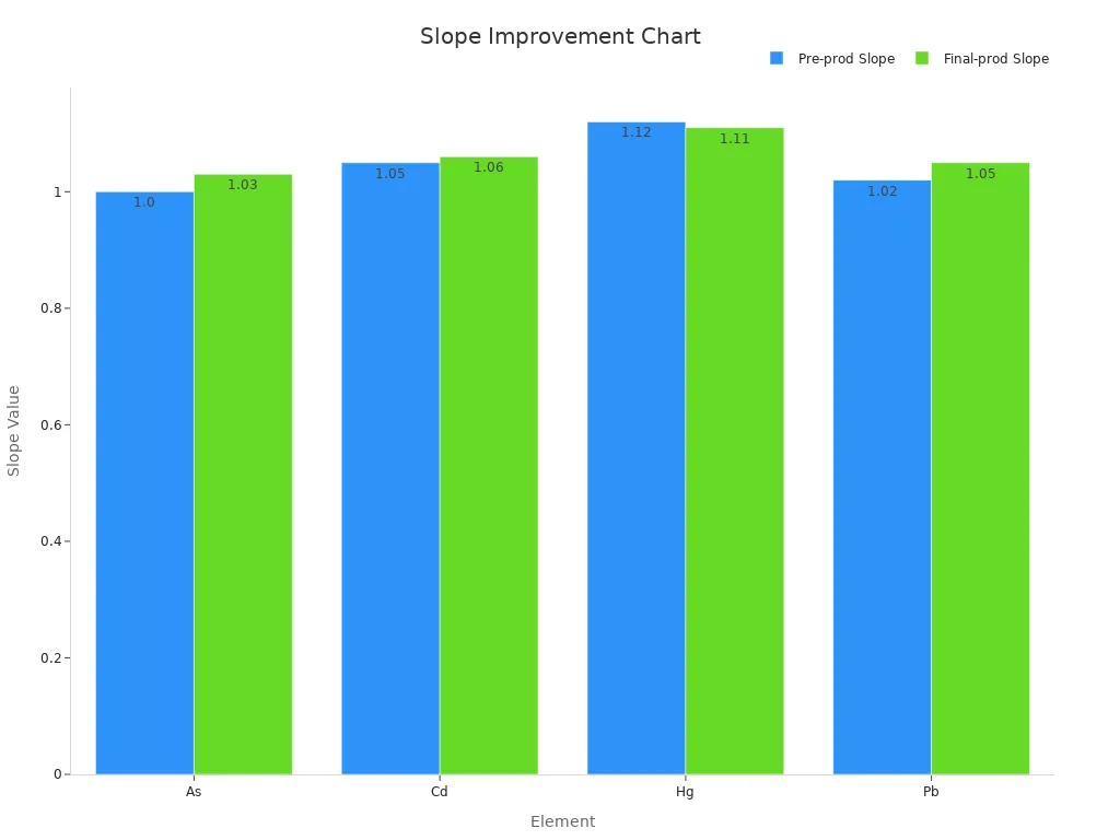
توضح هذه النتائج أن خوارزمية FP تعطي قياسات أكثر دقة وموثوقية بعد تحسينها.

إيجابيات وسلبيات

تحتوي خوارزمية FP على العديد من نقاط القوة لتحليل XRF:

• يعطي دقة جيدة, مع عدم اليقين النسبي للأفلام الرقيقة عادة بين 1% و 10%.

• يمكن أن تقيس العديد من العناصر في وقت واحد, حتى في عينات مع العديد من الطبقات أو الأجزاء.

• يحتاج إلى معايرة أقل من الأساليب الأخرى, لذلك يوفر الوقت والجهد.

• إنه يعمل بشكل جيد حتى لو لم يكن تخمينك الأول عن العينة مثاليًا.

لكن خوارزمية FP لديها أيضًا بعض الحدود:

• لا يعطي فترات ثقة إحصائية لنتائجها.

• لا يمكن التحقق مباشرة من العينات الرقيقة إذا كنت لا تعرف سمكها.

• إنه يعمل فقط للتركيبات الأولية, ليس للمركبات.

• لبعض الحالات الخاصة, مثل أفلام رقيقة جدا, قد تعمل الطرق الأخرى بشكل أفضل.

يلخص الجدول أدناه المزايا والحدود الرئيسية:

ملحوظة: تتطابق خوارزمية FP بشكل جيد مع طرق القياس الأخرى, مثل البروفيسري و SEM, إذا كنت تعرف كثافة العينة. تعني هذه الاتفاقية أنه يمكنك الوثوق بنتائج خوارزمية FP في العديد من حالات العالم الحقيقي.

طريقة المعامل التجريبي

كيف تعمل

تستخدم طريقة المعامل التجريبي قياسات حقيقية من المعايير لعمل منحنى المعايرة. يقيس العلماء شدة الأشعة السينية من العينات بكميات العناصر المعروفة. يرسمون هذه الأرقام ويستخدمون الانحدار الخطي لرسم خط يربط الشدة بالتركيز. غالبًا ما تبدو المعادلة هكذا:
Y = MX + E
حيث y هي الكثافة المقاسة, M هو المنحدر, x هو التركيز, و E هو التقاطع.

للحصول على نتائج جيدة, يتبع العلماء عدة خطوات. هم قياس شدة من المعايير بكميات العناصر المعروفة. أنها تصنع منحنى المعايرة باستخدام البيانات التي يجمعونها. يستخدمون تعداد الكثافة, مستويات الخلفية, وأرقام المعايرة مثل الميل والاعتراض كإحصائيات مهمة. يضيفون عوامل تصحيح لإصلاح تأثيرات المصفوفة والتداخلات. يقومون بإعداد العينات بعناية وأحيانًا يستخدمون عينة من الدوران لجعل العينة أكثر حتى. يفكرون في مدى عمق الأشعة السينية ومدى سمك العينة. يقارنون عينات غير معروفة بمنحنى المعايرة المحفوظة للعثور على التركيز.

هذه الطريقة تعمل بشكل جيد للعديد من المواد الجيولوجية, مثل الصخور البركانية وبلج. يساعد محلل XRF إعطاء نتائج قريبة من تلك من الأساليب القائمة على المختبر.

إيجابيات وسلبيات

طريقة المعامل التجريبي لها نقاط القوة والضعف على حد سواء. يعطي دقة جيدة وتكرار عندما يطابق نوع العينة معايير المعايرة. تستخدم الطريقة معاملات التأثير لإصلاح تأثيرات المصفوفة والذروة المتداخلة, مثل عندما تتداخل إشارات الزركونيوم والسترونتيوم. هذا التصحيح يجعل البيانات أفضل.

يوضح جدول أدناه نتائج رئيسية حول هذه الطريقة:

لكن الطريقة لها بعض الحدود. يمكن أن تكون منحنيات المعايرة بسيطة (خطي) أو أكثر تعقيدًا (متعدد الحدود). المنحنيات الخطية سهلة ولكن يمكن أن تتأثر بالقيم المتطرفة. منحنيات متعددة الحدود تناسب بشكل أفضل ولكن يمكن أن تنكسر بسهولة. القيم المتطرفة, مثل قيمة الزركونيوم العالية, يمكن تغيير النتائج. إزالتها تجعل الدقة أفضل ولكنها تجعل النطاق أصغر. يمكن أن تسبب القمم المتداخلة أخطاء إذا لم تكن ثابتة. تعتمد الطريقة على مدى جودة المعايير المرجعية ومدى جودة. لا يمكن أن يتنبأ بالنتائج للعينات خارج نطاق المعايرة. يجب أن تبقى إعدادات الأدوات وإعداد العينة كما هي.

ملحوظة: طريقة المعامل التجريبي تجعل النتائج أكثر تشابهًا بين الأدوات ولكن لا يمكنها التعامل مع عينات غير معروفة أو خارج نطاق المدى جيدًا. إنه يعمل بشكل أفضل للتحليل الروتيني مع أنواع العينات المعروفة.

مقارنة خوارزميات محلل XRF

دقة

تعطي خوارزمية FP دقة عالية للعديد من العينات. يستخدم القوانين الفيزيائية لإصلاح تأثيرات المصفوفة. هذا يساعده على قياس العناصر في العينات المختلطة. يمكن أن تكون طريقة المعامل التجريبي دقيقة أيضًا. لكنه يعمل بشكل جيد فقط إذا كانت العينة تتطابق مع المعايير. إذا كانت العينة مختلفة, قد لا تكون النتائج جيدة.

علم العلماء أن استخدام كل من خوارزمية FP والمعايرة التجريبية معًا يساعد أكثر. على سبيل المثال, عند الاختبار ذهب سبائك, عملت هذه الطريقة مجتمعة بشكل جيد للغاية. تتطابق القيم المقاسة والمعتمدة بشكل مثالي تقريبًا (r² = 0.9999). كان الخطأ النسبي أقل من 0.1%. هذا يعني أن الطريقة المشتركة يمكن أن تكون جيدة أو أفضل من طرق المختبر لبعض العناصر.

عندما تحتاج إلى أفضل دقة, عادة ما تكون خوارزمية FP أو الطريقة المشتركة أفضل. هذا صحيح بالنسبة للعينات غير المعروفة أو المختلطة.

معايرة

المعايرة مهمة لكلا الخوارزميات. تحتاج خوارزمية FP فقط إلى بعض العينات المرجعية. يستخدم الثوابت المادية, لذلك من الأسهل إعداد مواد جديدة. تحتاج طريقة المعامل التجريبي إلى العديد من المعايير التي تشبه العينات تمامًا. إذا كانت المعايير لا تتطابق, المعايرة لن تعمل بشكل جيد.

يوضح الجدول أدناه كيف تغير المعايرة النتائج:

يوضح الجدول أن استخدام كل من طرق المعايرة يقلل من الأخطاء. كما أنه يجعل النتائج أكثر جدارة بالثقة. خوارزمية FP وحدها لديها بالفعل أخطاء منخفضة. إضافة المعايرة التجريبية تجعلها أفضل.

سهولة الاستخدام

خوارزمية FP سهلة الاستخدام للعديد من العينات. لا يحتاج المستخدمون إلى وضع الكثير من المعايير. يمكنهم الحصول على النتائج بسرعة, حتى لو لم يعرفوا الكثير عن العينة. معظم محلل XRF يساعد البرنامج المستخدمين خطوة بخطوة.

تأخذ طريقة المعامل التجريبي المزيد من العمل. يجب على المستخدمين إنشاء العديد من المعايير وقياسها. يتعين عليهم أيضًا الحفاظ على إعدادات الأداة وتجربة الإعدادية في كل مرة. إذا تغير أي شيء, قد يحتاجون إلى إعادة المعايرة. هذا يستغرق المزيد من الوقت والجهد, خاصة بالنسبة للعينات الجديدة أو غير المعروفة.

لنفس النوع من العينة, يمكن أن تكون طريقة المعامل التجريبي بسيطًا. للعينات الجديدة أو المتغيرة, خوارزمية FP توفر الوقت وتساعد على تجنب الأخطاء.

المرونة

تعمل خوارزمية FP مع العديد من أنواع العينات. يمكنه التعامل مع مواد غير معروفة, الخلائط, وعينات الطبقات. يمكن للمستخدمين اختبار عينات مختلفة دون وضع منحنيات معايرة جديدة في كل مرة. هذا يجعل خوارزمية FP مرنة للغاية.

تعمل طريقة المعامل التجريبي بشكل أفضل عندما تتطابق العينة مع المعايير. إذا تغيرت العينة, يجب على المستخدمين إنشاء منحنيات معايرة جديدة. هذا يجعلها أقل فائدة للعينات غير المعروفة أو المعقدة.

مقارنة سريعة:

• خوارزمية FP

  • يعالج تأثيرات المصفوفة بشكل جيد

  • يحتاج إلى معايرة أقل

  • يعمل للعينات غير المعروفة والمعقدة

  • يحتاج إلى بعض الفهم للنماذج المادية

• طريقة المعامل التجريبي

  • يعمل بشكل أفضل للروتين, عينات معروفة

  • يحتاج إلى العديد من المعايير لكل نوع عينة

  • ليست جيدة للعينات غير المعروفة أو المتغيرة

  • الرياضيات البسيطة, لكن أقل مرونة

لتلخيص, خوارزمية FP أكثر مرونة ودقيقة لمعظم وظائف محلل XRF. طريقة المعامل التجريبي مفيد للعمل الروتيني مع عينات مستقرة.

استخدام العالم الحقيقي

الحالات الصناعية

تستخدم العديد من الشركات تحليل XRF لإصلاح المشكلات الحقيقية. في تشانغشون, الصين, قام مجموعة بفحص تربة المدينة للمعادن الثقيلة باستخدام XRF المحمولة. لقد عملوا في منطقة مزدحمة مع الكثير من المصانع. استخدمت المجموعة أ نموذج الرياضيات الخاص لإصلاح بيانات XRF. هذا جعل نتائجهم جيدة مثل الاختبارات المعملية. يمكنهم التحقق من العديد من الأماكن بسرعة وتكوين التلوث على الفور. هذا يدل على مساعدة خوارزميات XRF في السرعة, شيكات كبيرة.

مثال آخر من البرتغال. نظر العلماء إلى التربة بالقرب من مناجم الفحم القديمة. استخدموا الرياضيات المتقدمة مع بيانات XRF للعثور على معادن مثل الزرنيخ والرصاص. أعطت طريقتهم نتائج قوية, مع R² القيم من 0.79 ل 0.99 لعناصر مختلفة. هذه الأرقام العالية تعني أن تحليل XRF عملت بشكل جيد, حتى في الأماكن القذرة. جعلت الخوارزمية الصحيحة محلل XRF أداة قوية للصناعة والبيئة.

المختبر والحقل

يقوم الباحثون أيضًا باختبار خوارزميات XRF في المختبرات وخارجها. في دراسة واحدة, استخدمت الفرق XRF المحمولة على الزجاج القديم من المواقع الأثرية. على الرغم من أن الآلات كانت مختلفة, حصلوا على نتائج مماثلة عن طريق إصلاح بيانات FP. عندما كان لديهم فقط عدد قليل من المعايير, استخدموا تصحيحات نسبة. مع المزيد من المعايير, استخدموا الانحدار الخطي. هذا جعل النتائج أفضل وساعد في مقارنة البيانات من مختبرات مختلفة.

في دراسة مختبر أخرى, اختبر العلماء سبائك المعادن الثمينة. وجدوا أن الأساليب التجريبية تحتاج إلى العديد من معايير المطابقة وأسطح العينات السلسة. عملت طريقة FP بشكل أفضل عندما كانت المعايير مفقودة أو أن العينات لم تكن مثالية. باستخدام FP مع المعايرة التجريبية, لقد حصلوا على نتائج تتطابق مع قيم معتمدة, مع الأخطاء تحت 0.1%. بهذه الطريقة جعلت كل من الدقة والثقة بشكل أفضل, إن إظهار سبب استخدام كلتا الطريقتين في العينات المعقدة.

اختيار محلل XRF الخاص بك

متى تستخدم FP

خوارزمية FP هي الأفضل عندما تحتاج إلى اختبار أنواع كثيرة من العينات. يستخدم النماذج المادية, لذلك لا تحتاج إلى الكثير من معايير المعايرة. إنه يعمل بشكل جيد مع عينات غير معروفة أو طبقات. تستخدم العديد من الشركات خوارزمية FP في إعدادات مضان الأشعة السينية الدقيقة متحد البؤر. تساعد هذه الإعدادات في صنع خرائط ثلاثية الأبعاد للعناصر في مواد ذات طبقات أو منظمة. على سبيل المثال, تستخدم الشركات FP للتحقق من عينات البوليمر متعددة الطبقات مع مواد الحديد الحديد. يستخدم العلماء FP لدراسة الأشياء الفنية, مثل الطبقات أو الرق, دون إتلافهم. يستخدم علماء الجيولوجية FP لرسم خريطة للضواحي في الماس أو المعادن. يستخدم الباحثون FP لتتبع العناصر الغذائية النباتية في العينات البيولوجية. طريقة FP جيدة أيضًا عندما يصعب العثور على مواد مرجعية. إنه يعمل بشكل جيد للعينات ذات الأرقام الذرية الخفيفة أو المتوسطة, مثل البوليمرات أو المواد العضوية. يمكن للمستخدمين الوثوق في خوارزمية FP للحصول على نتائج شبه كمية, خاصة عندما يكون شكل العينة صعبًا.

نصيحة: اختر FP إذا كنت بحاجة إلى اختبار غير معروف, طبقة, أو عينات منظمة, أو إذا لم يكن لديك معايير مطابقة للمصفوفة.

متى تستخدم التجريبية

طريقة المعامل التجريبي هي خيار جيد للاختبارات الروتينية للعينات التي تعرفها جيدًا. تستخدم هذه الطريقة منحنيات المعايرة المصنوعة من المعايير التي تتطابق مع مصفوفة العينة. إنه يعمل بشكل جيد متى تأثيرات المصفوفة, مثل التألق الثانوي أو الامتصاص, قوية ويمكن إصلاحها مع الانحدار. تظهر الدراسات طرقًا تجريبية, مثل الانحدار الخطي المتعدد والطرق الكيميائية, غالبًا ما يعمل بشكل أفضل من FP في المصفوفات المعقدة مثل الفولاذ, خامات, أو الزجاج القديم. الأساليب التجريبية تتعامل مع تأثيرات المصفوفة والتدخلات الطيفية بشكل أفضل إذا كان لديك بيانات معايرة كافية. أنها تعطي دقة عالية للعينات ذات المصفوفات المعقدة أو المختلطة, طالما أن عينات المعايرة تتطابق مع المجهولين. الطرق الكيميائية, يحب المربعات الصغرى الجزئية, ساعد في الحصول على نتائج أفضل في عينات صعبة. يجب على المستخدمين اختيار الطريقة التجريبية عندما يكون لديهم العديد من معايير المطابقة ويحتاجون إلى التحكم في تأثيرات المصفوفة في المواد المعقدة.

ملحوظة: استخدم الطريقة التجريبية للروتين, عمل عالي الدقة مع معروف, عينات معقدة وعندما يمكنك وضع معايير معايرة كافية.

قائمة مراجعة القرار

استخدم قائمة المراجعة هذه لمساعدتك في اختيار الخوارزمية المناسبة لك محلل XRF:

• هل عيناتك غير معروفة, طبقة, أو منظم? → FP

• ألا تملك معايير المعايرة المطابقة للمصفوفة? → FP

• هل تحتاج إلى اختبار البوليمرات, بيولوجي, أو عينات من الفن التاريخي? → FP

• هل عيناتك معروفة والمعايير سهلة الحصول عليها? → تجريبي

• هل تؤثر تأثيرات المصفوفة أو التدخلات الطيفية على تغيير نتائجك كثيرًا? → تجريبي

• هل تحتاج إلى أفضل دقة في المجمع, عينات مختلطة? → تجريبي

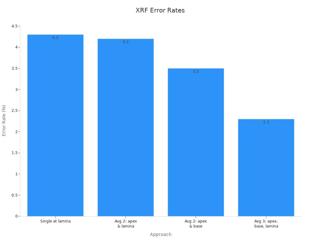
خوارزمية FP دقيقة للغاية وتعمل مع العديد من العينات. الطريقة التجريبية هي الأفضل للعينات التي تعرفها جيدًا. يجب عليك اختيار الطريقة التي تناسب العينة وما تحتاجها. فكر في مدى صعوبة عينتك, ما هي أدوات المعايرة التي لديك, وكيف تريد أن تكون دقيقًا. بعض الطرق المتقدمة, مثل TXRF, يمكن أن تجد كميات صغيرة جدًا. يمكنهم قياس أقل 10grams ⁻². هذا رائع للأفلام الرقيقة والتحقق من الأسطح. الرسم البياني أدناه يوضح أن أخذ المزيد من القياسات يمكن أن يجعل الأخطاء تنخفض في تحليل XRF.

إذا كنت تريد معرفة المزيد, يمكنك النظر في طرق التحليل الديناميكي. يمكنك أيضًا تجربة برنامج مفتوح المصدر مثل Geopixe.

التعليمات

ما هو الفرق الرئيسي بين خوارزمية FP وطريقة المعامل التجريبي?

ال خوارزمية FP يستخدم الفيزياء والرياضيات لدراسة العينات. تستخدم طريقة المعامل التجريبي قياسات حقيقية من المعايير المعروفة. FP مفيد للعينات التي لا تعرفها الكثير عنها. الطريقة التجريبية تعمل بشكل أفضل للعينات التي تعرفها جيدًا بالفعل.

هل يمكن للمستخدمين التبديل بين FP والطرق التجريبية على نفس محلل XRF?

الأكثر جديدة تحليلات XRF اسمح للمستخدمين باختيار أي من الطريقة. يعتمد التبديل على البرنامج وكيفية إعداد المعايرة. يجب على المستخدمين النظر في دليل المحلل لمعرفة كيفية التبديل.

لماذا تحتاج خوارزمية FP إلى عدد أقل من معايير المعايرة?

تستخدم خوارزمية FP القوانين الفيزيائية وعدد قليل من العينات المرجعية. لا يحتاج إلى العديد من المعايير لأنه يكتشف نتائج من خلال كيفية تفاعل الأشعة السينية مع العناصر.

هل يؤثر تحضير العينة على كلا الخوارزميات?

نعم. كلا الخوارزميات تعمل بشكل أفضل مع نظافة, مستوي, وحتى العينات. إذا لم تحضر العينات بشكل جيد, يمكن أن تعطي كلتا الطريقتين نتائج خاطئة.

الطريقة الأفضل للتحليل الميداني?

عادة ما تكون خوارزمية FP أفضل للعمل الميداني. يمكنه التعامل مع عينات غير معروفة أو مختلطة ولا تحتاج إلى الكثير من المعايرة. هذا يجعل الأمر أسهل وأسرع لفحص سريع خارج المختبر.